Drive shaping workflow
Drive shaping builds the time-dependent drive Hamiltonian — amplitude and detuning waveforms, and optionally a detuning map — applied to a register during quantum solving. Each drive shaping algorithm is callable directly, or picked and configured through Solver/SolverConfig.
Goal of drive shaping
The embedding step encodes the QUBO's off-diagonal coefficients \(Q_{ij}\) into the physical interaction between atoms. The diagonal coefficients \(Q_{ii}\) are encoded separately, as local detunings \(\delta_i\) applied to each atom: \(Q_{ii} \longleftrightarrow -2\delta_i\) (see The quantum pipeline). Drive shaping is the step that builds this detuning schedule, together with the amplitude (Rabi frequency) schedule that drives the system, so that the ground state of the resulting Hamiltonian encodes a good solution of the QUBO.
A drive shaping algorithm returns a qoolqit.Drive — an amplitude waveform, a detuning waveform, and optionally a per-atom weighted detuning (a Detuning Map Modulator, or DMM) for site-dependent control — together with a Solution. Algorithms that only build the drive analytically from the problem's structure return an empty Solution, since no sampling has happened yet; algorithms that also run a quantum simulation internally return a populated one.
qubosolver currently ships three drive shaping algorithms — proportional-diagonal, local-energy-scale, and Bayesian search, described below — plus the option to write your own.
Proportional-diagonal
The proportional-diagonal shaper builds a fixed drive directly from the diagonal of the QUBO matrix, without any numerical optimization: the final local detuning \(\delta_i(T)\) is set proportional to \(-Q_{ii}\), and the peak Rabi frequency \(\Omega_{\max}\) is set proportional to the peak detuning via a kappa coefficient.
- API reference:
qubosolver.drive_shaping.proportional_diagonal - Tutorial: Proportional-diagonal notebook
- Under the hood: Proportional-diagonal
Code example
from qubosolver import Instance, matrix, embedding, drive_shaping
import qoolqit

# Private utility to set seed.
from qubosolver.utils._random import manual_seed

manual_seed(958)

instance = Instance(
    matrix.tensor(
        [
            [-1, 1, 2, 1],
            [1, -3, 3, 0],
            [2, 3, -1, 5],
            [1, 0, 5, -2],
        ]
    )
)
device = qoolqit.AnalogDeviceWithDMM()
register = embedding.blade.embed_for_device(instance, device)

drive = drive_shaping.proportional_diagonal.build_drive(
    instance, register, device=device, dmm=True, kappa=0.25
)
print(drive)
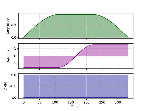
Local-energy-scale
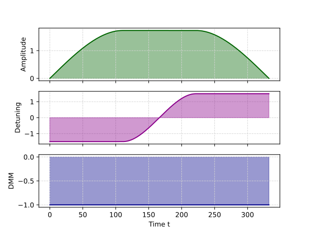
The local-energy-scale shaper also builds a fixed drive analytically, but derives the peak Rabi frequency from the average local physical energy scale \(E_i = |\delta_i(T)| + \sum_{j \neq i} |V_{ij}|\) — combining the target detuning with the interaction strengths induced by the embedded register — rather than from the detuning alone.
- API reference:
qubosolver.drive_shaping.local_energy_scale - Tutorial: Local-energy-scale notebook
- Under the hood: Local-energy-scale
Code example
from qubosolver import Instance, matrix, embedding, drive_shaping
import qoolqit

# Private utility to set seed.
from qubosolver.utils._random import manual_seed

manual_seed(958)

instance = Instance(
    matrix.tensor(
        [
            [-1, 1, 2, 1],
            [1, -3, 3, 0],
            [2, 3, -1, 5],
            [1, 0, 5, -2],
        ]
    )
)
device = qoolqit.AnalogDeviceWithDMM()
register = embedding.blade.embed_for_device(instance, device)

drive = drive_shaping.local_energy_scale.build_drive(
    instance, register, device=device, dmm=True, kappa=0.25
)
print(drive)
Bayesian search
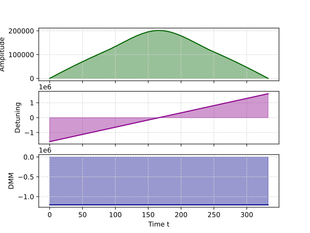
Unlike the two heuristics above, Bayesian search is not really a drive-shaping algorithm — it is a hybrid quantum-classical solver in its own right: it runs a Bayesian optimization loop (skopt.gp_minimize) over six waveform knots (three for the amplitude, three for the detuning), running a quantum simulation at each evaluation and minimizing a configurable objective of the resulting Solution. Because that loop already produces both a tuned drive and a sampled solution, it can also be reused as a drive shaper for another solving step — which is why it is included here.
This dual role means it is more expensive than the other two heuristics, but able to adapt the drive to the problem and the backend rather than following a fixed rule. Because it simulates the problem while shaping the drive, it needs a backend in addition to the device, and it returns a populated Solution alongside the drive — reused directly if you're also using it as your solving step.
- API reference:
qubosolver.solving.drive_bayesian_search - Tutorial: Bayesian search notebook
- Under the hood: Bayesian search
The example below uses a small n_evaluations for a quick, self-contained doc run; see solving.drive_bayesian_search.Config for the full set of parameters, including the initial waveform knots, the random seed, and the objective function.
Code example
from qubosolver import Instance, matrix, embedding, solving, analysis, LocalEmulator
import qoolqit

# Private utility to set seed.
from qubosolver.utils._random import manual_seed

manual_seed(958)

instance = Instance(
    matrix.tensor(
        [
            [-1, 1, 2, 1],
            [1, -3, 3, 0],
            [2, 3, -1, 5],
            [1, 0, 5, -2],
        ]
    )
)
device = qoolqit.AnalogDeviceWithDMM()
backend = LocalEmulator()

register = embedding.blade.embed_for_device(instance, device)

config = solving.drive_bayesian_search.Config(n_evaluations=11)

solution, drive = solving.drive_bayesian_search.solve(
    instance, register, backend=backend, device=device, dmm=True, config=config
)
print(analysis.to_dataframe([solution]))
Custom drive
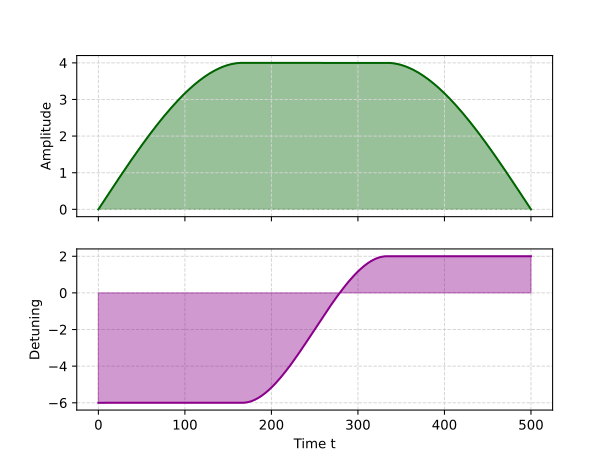
You can skip the built-in algorithms altogether and build a qoolqit.Drive directly from waveforms, as in the example below, or reuse a drive computed elsewhere:
import qoolqit
from pathlib import Path
from matplotlib import pyplot as plt

drive = qoolqit.Drive(
    amplitude=qoolqit.InterpolatedWaveform(500, [1e-9, 4.0, 4.0, 1e-9]),
    detuning=qoolqit.InterpolatedWaveform(500, [-6.0, -6.0, 2.0, 2.0]),
)

output_dir = Path.cwd()
output_dir.mkdir(parents=True, exist_ok=True)

drive.draw()
fig = plt.gcf()
fig.savefig(output_dir / "quantum_drive_shaping_custom_drive.svg")
plt.close(fig)
The Solver shortcut
Rather than calling drive_shaping.proportional_diagonal.build_drive, drive_shaping.local_energy_scale.build_drive, or solving.drive_bayesian_search.solve directly, you can select and configure the drive shaping algorithm through DriveShapingConfig, nested in QuantumSolvingConfig and SolverConfig; Solver then runs it as part of the full quantum pipeline. Leaving DriveShapingConfig unset falls back to the proportional-diagonal shaper with DMM enabled — see SolverConfig for the full set of defaults.
DriveShapingConfig only exposes the most commonly tuned parameters of each algorithm (e.g. proportional_diagonal_kappa, local_energy_scale_kappa, bayesian_search_n_calls). Finer-grained parameters — such as Bayesian search's objective_fn or its optimization callback — are not settable this way; call solving.drive_bayesian_search.solve directly with a full solving.drive_bayesian_search.Config if you need those.
```python exec="on" source="tabbed-left" session="drive_shaping" result="text" from qubosolver import SolverConfig, QuantumSolvingConfig, DriveShapingConfig from dataclasses import asdict import pprint
drive_shaping_config = DriveShapingConfig( algorithm="local_energy_scale", # algorithm = "proportional_diagonal", # algorithm = "bayesian_search", dmm=True, local_energy_scale_kappa=0.3, ) quantum_config = QuantumSolvingConfig( drive_shaping=drive_shaping_config, ) solver_config = SolverConfig( solving=quantum_config, ) print(pprint.pformat(asdict(solver_config.solving.drive_shaping))) ```