Embedding workflow
Embedding maps a QUBO instance's variables onto atom positions on a quantum device, so that the physical interaction between atoms approximates the QUBO's coefficients. Each embedding algorithm is callable directly, or picked and configured through Solver/SolverConfig.
Goal of embedding
Solving a QUBO on a neutral-atom quantum device requires translating the problem's coefficients into a physical layout of atoms. Each QUBO variable \(i\) is represented by an atom, placed at some position on the device. The interaction strength between two atoms is a function of the physical distance between them (typically decaying with distance, e.g. as \(1/r^6\) for Rydberg interactions), whereas the QUBO matrix specifies the desired coupling strength \(Q_{ij}\) between each pair of variables \(i\) and \(j\).
The goal of embedding is therefore to find atom positions such that the interaction strengths induced by their pairwise distances reproduce, as closely as possible, the couplings encoded in the QUBO matrix — subject to the constraints of the target device (register size, minimal distance between atoms, layout geometry, etc.). A good embedding is what allows the quantum device to encode the optimization problem faithfully, so that its ground state (or low-energy states) correspond to good solutions of the original QUBO.
Because the induced interaction \(J_{ij} \propto 1/r_{ij}^6\) is always positive, an embedding can only reproduce non-negative off-diagonal couplings. QUBO matrices with negative off-diagonal coefficients cannot be embedded directly; see Negative coefficient preprocessing for how such coefficients are eliminated or zeroed out before embedding.
Since embedding is an approximation, it is worth having a way to judge how good it is. The relative norm error between the QUBO matrix and the induced interaction matrix (shown in the examples below) is the most direct such proxy, and cheap to compute. But it is only a proxy: what actually matters is whether the embedding leads the quantum device to good solutions of the original QUBO, and a lower matrix error does not always mean a better solution — e.g. a small number of badly reproduced couplings on variables that matter more to the optimum can hurt more than a uniformly larger error spread evenly across all pairs.
See the embedding overview notebook for a hands-on introduction to this step.
qubosolver currently ships two embedding algorithms — BLaDE and greedy layout, described below — plus the option to write your own embedding function or supply a precomputed register.
Warning
Each algorithm exposes two entry points: embed(instance, config=...) and embed_for_device(instance, device). embed takes a fully-resolved config as-is and does not look at any device, so use it to tune parameters freely — but tread carefully with device-dependent ones: a value unsuited to your target device can produce a register that device cannot realize. embed_for_device derives those device-dependent fields automatically and is the safer default whenever you have a target device. See the API reference for the exact fields each algorithm derives.
BLaDE
BLaDE places atoms by progressively projecting the problem from a high-dimensional layout down to the device's 2D plane, refining positions layer by layer so that pairwise distances keep approximating the QUBO couplings at each step.
- API reference:
qubosolver.embedding.blade - Tutorial: BLaDE notebook
- Under the hood: BLaDE
The example below runs BLaDE sized for a target device via embed_for_device — the sequence of dimension layers, number of steps per round, and starting positions can all be tuned by combining embedding.blade.Config(device=...) with embed directly. See Qoolqit's documentation for the available parameters.
Code example
from qubosolver import Instance, matrix, embedding
import torch
import qoolqit

# Private utility to set seed.
from qubosolver.utils._random import manual_seed

manual_seed(958)

instance = Instance(
    matrix.tensor(
        [
            [0, 1, 2, 1],
            [1, 0, 3, 0],
            [2, 3, 0, 5],
            [1, 0, 5, 0],
        ]
    )
)
register = embedding.blade.embed_for_device(instance, qoolqit.AnalogDevice())
interaction_matrix = matrix.as_tensor(register.interaction_matrix())

torch.set_printoptions(precision=2)
print(f"QUBO matrix:\n{instance.matrix}\n")
print(f"Interaction matrix:\n{interaction_matrix}\n")

relative_error = 100 * (instance.matrix - interaction_matrix).norm() / instance.matrix.norm()
print(f"Relative error = {relative_error:.2f} %")
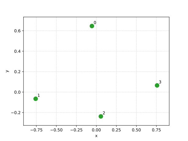
Note that by default, before running BLaDE, the positions are initialized using MDS (Multi-Dimensional Scaling). You can disable that by instantiating a config with
embedding.blade.Config(initialize_with_mds=False).
Greedy embedder
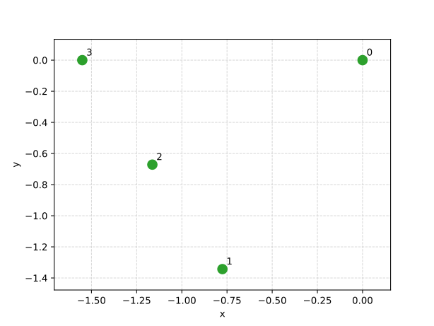
The greedy embedder picks atom positions from a fixed lattice of candidate trap sites (triangular or square), assigning variables one at a time to the site that best matches their required couplings to already-placed variables.
- API reference:
qubosolver.embedding.greedy_layout - Tutorial: Greedy layout notebook
- Under the hood: Greedy Layout
Code example
from qubosolver import Instance, matrix, embedding
import torch
import qoolqit

# Private utility to set seed.
from qubosolver.utils._random import manual_seed

manual_seed(851)

instance = Instance(
    matrix.tensor(
        [
            [0, 1, 2, 1],
            [1, 0, 3, 0],
            [2, 3, 0, 5],
            [1, 0, 5, 0],
        ]
    )
)

register = embedding.greedy_layout.embed_for_device(
    instance,
    qoolqit.AnalogDevice(),
)
interaction_matrix = matrix.as_tensor(register.interaction_matrix())

torch.set_printoptions(precision=2)
print(f"QUBO matrix:\n{instance.matrix}\n")
print(f"Interaction matrix:\n{interaction_matrix}\n")

relative_error = 100 * (instance.matrix - interaction_matrix).norm() / instance.matrix.norm()
print(f"Relative error = {relative_error:.2f} %")
Custom register
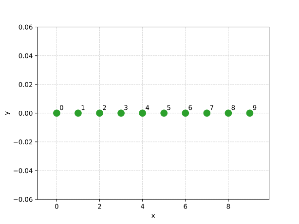
You can skip embedding algorithms altogether and build a qoolqit.Register directly from coordinates, as in the example below, or reuse a register computed elsewhere or encode problem-specific knowledge about where atoms should sit:
import qoolqit
from pathlib import Path
from matplotlib import pyplot as plt

coords = [[i, 0] for i in range(10)]
register = qoolqit.Register.from_coordinates(coords)

output_dir = Path.cwd()
output_dir.mkdir(parents=True, exist_ok=True)

register.draw()
fig = plt.gcf()
fig.savefig(output_dir / "quantum_embedding_custom_register.svg")
plt.close(fig)
The Solver shortcut
Rather than calling embedding.blade.embed or embedding.greedy_layout.embed directly, you can select and configure the embedding algorithm through EmbeddingConfig, nested in QuantumSolvingConfig and SolverConfig; Solver then runs it as part of the full quantum pipeline. Leaving EmbeddingConfig unset falls back to the BLaDE embedder — see SolverConfig for the full set of defaults.
EmbeddingConfig only exposes the most commonly tuned parameters of each algorithm (e.g. blade_steps_per_round, greedy_layout_lattice). Finer-grained parameters — such as BLaDE's pca flag or its compute_* schedule functions — are not settable this way; call embedding.blade.embed/embedding.greedy_layout.embed directly with a full blade.Config/greedy_layout.Config if you need those.
from qubosolver import SolverConfig, QuantumSolvingConfig, EmbeddingConfig
from dataclasses import asdict
import pprint

embedding_config = EmbeddingConfig(
    algorithm="blade",
    # algorithm = "greedy_layout",
    # greedy_layout_lattice = "triangular",
    greedy_layout_lattice="square",
)
quantum_config = QuantumSolvingConfig(
    embedding=embedding_config,
)
solver_config = SolverConfig(
    solving=quantum_config,
)
print(pprint.pformat(asdict(solver_config.solving.embedding)))