Estimating Memory Consumption and Runtime
The presence of the max_bond_dim and max_krylov_dim config parameters means an upper bound on memory consumption and the complexity of the time evolving algorithm can be estimated. By limiting the max_bond_dim of a simulation to make it fit in the available hardware memory, it can be guaranteed to run for arbitrary times for an arbitrary number of qubits. Of course, the sources of error described on the error page imply that limiting the memory consumption of the program will negatively impact the quality of the results once a certain threshold is exceeded. The page in this link, for example, outlines a case study to determine whether emulation results are accurate.
Estimating the memory consumption of a simulation
In this section we outline how to estimate the memory consumption of a simulation, for a given max_bond_dim, a Krylov subspace of size max_krylov_dim, and for \(N\) being the number of qubits to be simulated.
There are four contributions to the peak memory consumption of emu-mps that will be discussed in the next sections:
- the state
- the baths
- the Krylov space
- temporary tensors
Contribution from the state
The quantum state is stored in MPS format (see here). At worst, the bond dimensions of the tensors in an MPS grow exponentially inwards as
in which case an MPS will take more memory than a state vector. Let \(\chi\) denote the value of max_bond_dim.
When \(\chi<2^{N/2}\), the bond dimensions in the center all cap at that fixed value of max_bond_dim. Since each tensor in the MPS has 2 bonds of size at most \(\chi\), and a physical index of size \(p=2\) in the qubit (\(2\)-level system) case, where each element in the tensor takes \(s=16\) bytes (\(2\) \(8\)-byte floats to store a complex number), the memory consumption of the state reads
and more generally,
for the qudit (p-level system) case.
Note that this is a strict over-estimation because the outer bonds in the MPS will be much smaller than \(\chi\), but it is asymptotically correct as \(N\rightarrow \infty\).
Contribution from the baths
For the currently available solvers (TDVP and DMRG), for each qubit a left and a right bath tensor is stored. The bath tensors are used to compute an effective interaction between the 2-qubit subsystem being evolved, and the rest of the system (see here). Each of them has 3 indices. Two of them will have a size that depends on the state that is evolved, here upper bounded by the maximum allowed value \(\chi\) for the bond dimension. For the third, the size \(h\) will depend on the interaction type. In concrete, for each qubit, \(h\) will be the bond dimension of the MPO representation of the Hamiltonian. In summary, for the Rydberg Hamiltonian we expect that \(h=3+n\), and for the XY Hamiltonian that \(h=4+2n\), where in both cases \(n=\text{min}(i,N-i-1)\) for the bath associated with the qubit \(i\). Assuming a constant, maximal, bond dimension for the state, the sum over all baths is an algebraic sum. For the Rydberg interaction it evaluates to:
Just as for the state this is a strict over-estimation that is asymptotically correct, because it assumes all the bonds in the state are of size \(\chi\). Note that the baths take up more memory than the state by a factor \(O(N)\), where the prefactor depends on the interaction type (for Rydberg it is \(1/8\)), making this term the most dominant for large qubit numbers. For this reason those baths which are not used in the Lanczos algorithm are always stored on CPU, even when the emulator is configured to use GPU. By overlapping the data transfers with other computations, we can avoid runtime impact at the cost of occasionally having a third bath tensor present on the GPU during the Lanczos algorithm. In this case we get
Contribution from the Krylov space
The remainder of the memory consumption is to compute the time-evolution of qubit pairs in the TDVP or DMRG algorithms. This is done by contracting 2 tensors from the MPS together into a single 2-qubit tensor, and time-evolving (or minimizing) it by applying an effective Hamiltonian constructed from the baths and the Hamiltonian MPO. Each 2-qubit tensor has a size bounded by \(sp^2\chi^2\), so the memory of the Krylov vectors used in the Lanczos algorithm reads
where \(k\) is the value of max_krylov_dim. Recall that the default value of \(k=100\) and if the Lanczos algorithm requires more Krylov vectors to converge to the tolerance, it will error, rather than exceed the above bound.
Contribution from temporary tensors
Finally, to compute the above Krylov vectors, the effective two-site Hamiltonian has to be applied to the previous Krylov vector to obtain the next one. The resulting tensor network contraction cannot be done in-place, so it has to store two intermediate results that get very large. Additionally, the contraction requires storage of a permuted copy of one the two bath tensors. The intermediate results take the most memory at the center qubit, where the bond dimension of the Hamiltonian becomes \(h\). At this point,
It should be noted that the value of \(h\) cited above assumes that all qubits in the system interact via a two-body term, which is technically true for the Rydberg interaction. However, small terms in the interaction matrix can be truncated away via a configuration option, and this will save memory.
Benchmarking memory footprint
Putting all of this together, for the total memory consumption \(m\) of the program, we can write the following bound for the CPU:
The quadratic scaling in \(N\) is due to the bath contribution. On the GPU, we get a linear scaling instead:
In this case, there is of course a quadratic scaling in the consumption of CPU RAM. For large system sizes, this will outstrip the memory requirements on the GPU, and it becomes important to ensure enough RAM is available for the program to run.
Note that these estimates are pessimistic, since not all \(k\) Krylov vectors are likely to be needed, and not all tensors in \(\psi\) and the baths have the maximum bond dimension \(d\). On the other hand, the estimate for \(|intermediate|\) is likely to be accurate, since the bond dimension of \(\chi\) is probably attained at the center qubit if the sequence is long enough.
Both TDVP and DMRG rely on the same bath construction and effective Hamiltonian machinery, so their memory requirements are expected to scale similarly with \(N\) and \(\chi\).
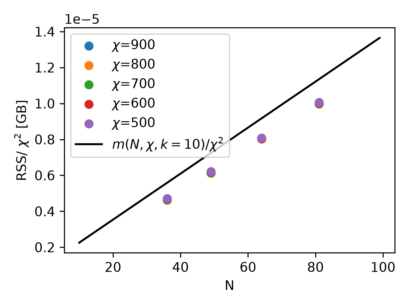
To test the accuracy of the above memory estimations, we benchmarked the TDVP algorithm by fixing the bond dimension to a particular desired value. We ran the benchmark on GPU, and consider the memory burden on the GPU.
For different combinations of the number of atoms in a register \(N\) and the fixed bond dimension \(\chi\), we collect the maximum resident set size, or RSS, on the GPU, which is expected to capture the maximum memory needed to run the emulation. We plot the RSS in the following picture (left), as a function of the number of qubits and for different bond dimensions. Notice that, once the RSS is normalized by \(\chi^2\), as suggested by our estimate above, all the points fall into the same functional dependency on the number of atoms. Moreover, as we plot the normalized function \(m(N,\chi,k)/\chi^2\), for a reasonable estimate of the size of the Krylov subspace (\(k=10\)), it is clear that our upper bound on memory occupation can be reasonably trusted on a wide range of system sizes and bond dimensions.
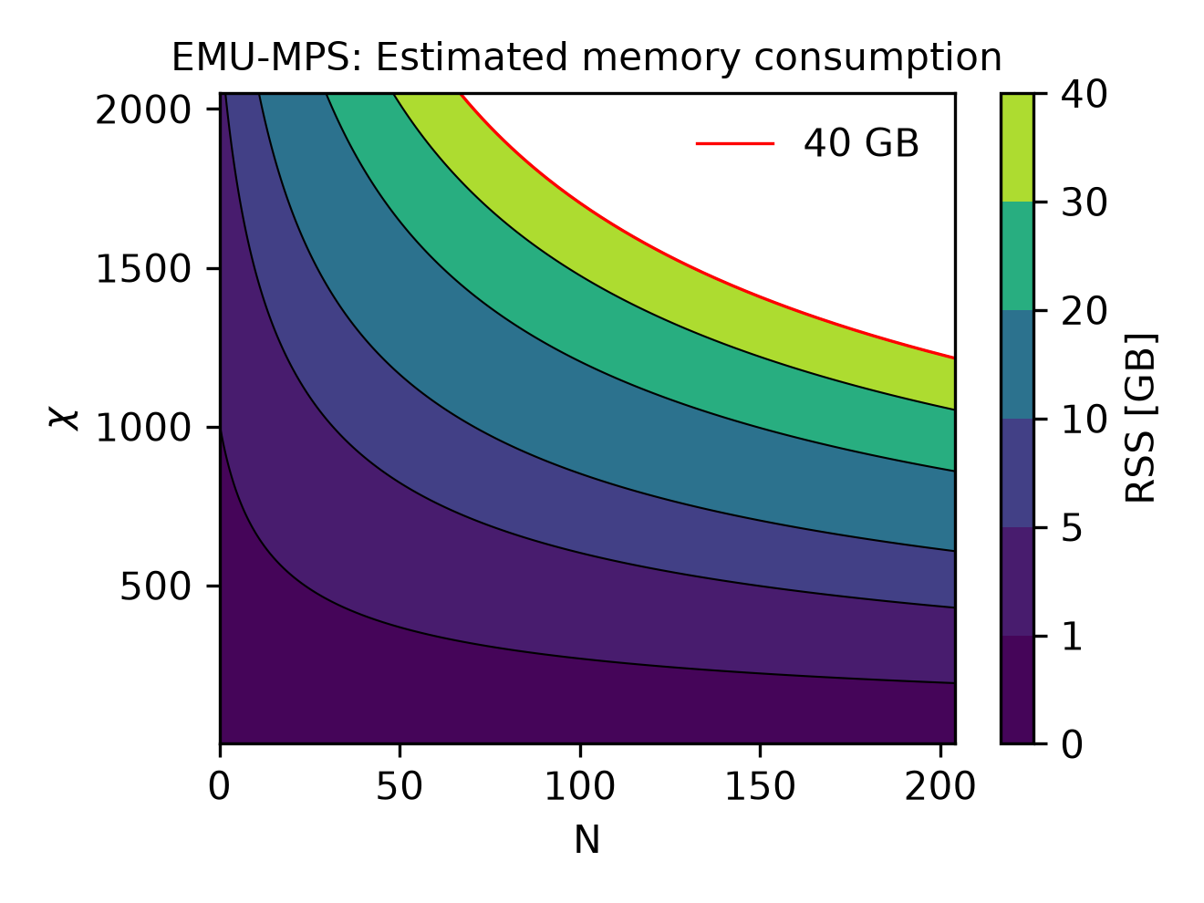
Finally, having established an estimate for the memory consumption, it makes sense to explore what are the available regimes of qubits/bond dimension can be reached for a given hardware capability. Since all heavy simulations will be run on an NVIDIA A100 (on Pasqal's DGX cluster), we have \(40\) GB of available memory. Therefore, above, we show (right image) the contour lines of the RSS estimate \(m(N,\chi,k=10) < 40\) GB for particular useful values of the total memory, allowing to quickly estimate the memory footprint of an emu-mps emulation.
Although these results are shown for TDVP, a similar analysis could be performed for DMRG, and we expect the resulting memory scaling to be comparable.
An example
For example, the results from the case study were obtained using \(N=49\) and \(d=1600\). Taking the above formula for GPU, we find a memory consumption of \(16.998\) GB even for \(k=0\), while the actual cited memory consumption on GPU is \(14.659\) GB. The actual number of Krylov vectors required to reach convergence is likely around 10, but this contribution is not visible since \(\psi\) and \(|\mathrm{bath}|\) are over-estimated.
Estimating the runtime of a simulation
Similarly to the previous section, here, we briefly estimate the complexity of both the two-site TDVP and DMRG algorithms we use to time evolve or minimize the state in a single pulse sequence step. As before, the two relevant computational steps are
- Computing the baths
- Applying the effective Hamiltonian
In both cases, it will boil down to an exercise in complexity estimation of tensor network contractions. For simplicity, as before, we will restrict to the worst case scenario in which the bond dimension \(\chi\) always take the maximum allowed value. Importantly, another significant contribution to the runtime can come from computing complex observables like two-point correlation functions, which is not included here.
Contribution from the baths
Roughly, baths computation involves the represented tensor network contraction:

Each of these tensor multiplication takes respectively \(O(ph\chi^3)\), \(O(p^2h^2\chi^2)\), and \(O(ph\chi^3)\). In an all-to-all Rydberg interaction, we already argued that the bond dimension of the Hamiltonian MPO should scale as the number of atoms. Moreover, the left and right baths need to be computed roughly N times, thus the overall expected complexity is \(O(N^2\chi^3) + O(N^3\chi^2)\).
Contribution from the effective Hamiltonian
Applying the effective two-body Hamiltonian is slightly a more involved tensor network contraction:

In steps, it is composed by applying:
- the left bath: \(O(p^2h\chi^3)\)
- a two-body term coming form the MPO Hamiltonian: \(O(p^4h^2\chi^2)\)
- the right bath: \(O(p^2h\chi^3)\)
As before, for an all-to-all Rydberg interaction we expect \(h\sim N\). Moreover, the effective Hamiltonian application needs to be done \(k\) times, to build the appropriate Krylov subspace, and for every pair. Finally, to complete the time evolution or the energy minimization and bring back the tensors of the state into an MPS form, a final singular value decomposition is required. For every pair, this requires \(O(N\chi^3)\) to be done. Overall, the expected complexity is thus \(O(kN^2\chi^3) + O(kN^3\chi^2) + O(N\chi^3)\).
Benchmarking runtime
From the previous complexity estimations, we expect the computational complexity of both the two-site TDVP and DMRG algorithms to have two main contributions
As previously discussed, both algorithms rely on the same bath construction and effective Hamiltonian machinery, so their scaling with the system size \(N\) and bond dimension \(\chi\) should be comparable.
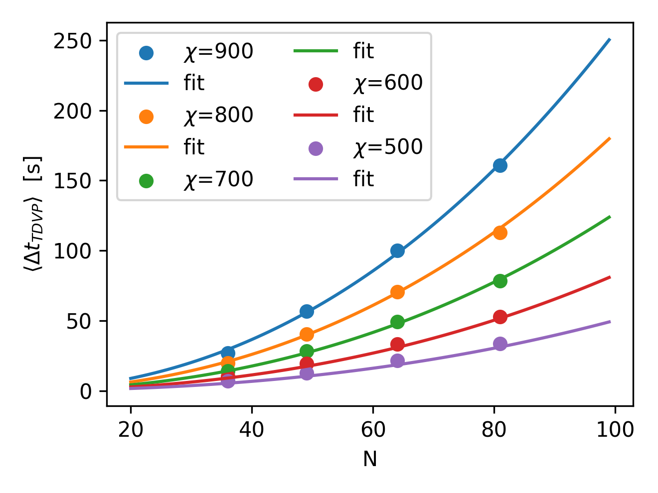
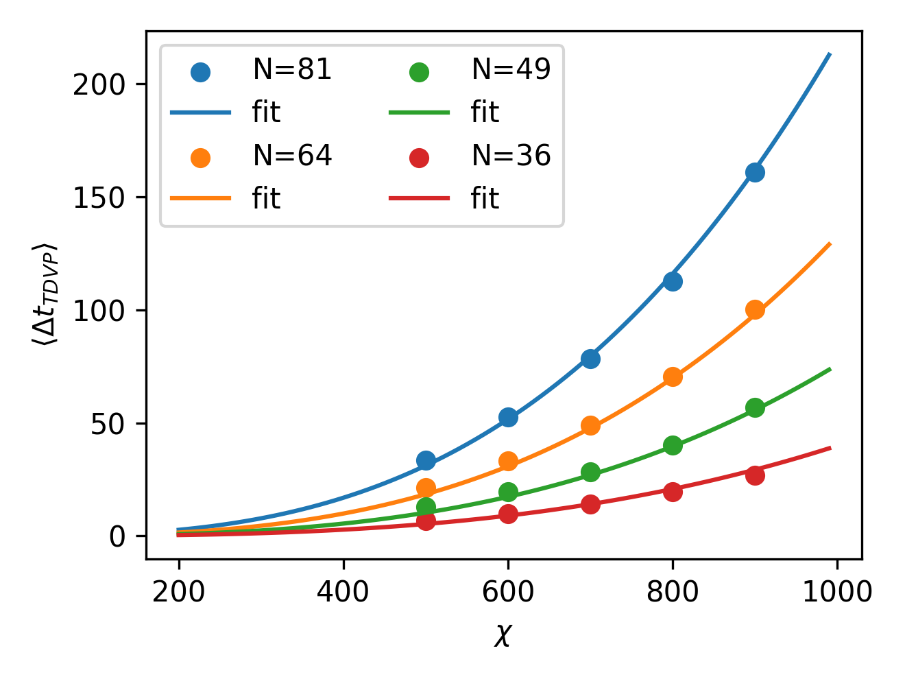
The study below focuses on TDVP, where we ran multiple simulations and measured the average runtime per time step. A similar analysis could be carried out for DMRG, and we expect it to lead to similar results.
Below, we show the obtained results for different number of atoms in a register \(N\) at fixed bond dimension \(\chi\) (left), and at different fixed \(N\) but increasing the bond dimension (left). On top of these data points, we also plot the resulting fit of the complexity estimation presented in the equation above. Remarkably, with just two parameters \(\alpha\) and \(\beta\) with get good agreement.
To wrap up, and to provide a practical tool for runtime estimation for emu-mps, the time required to perform a single time step in a sequence can be conveniently visualized (below) for both \(N\) and \(\chi\) on contour lines.
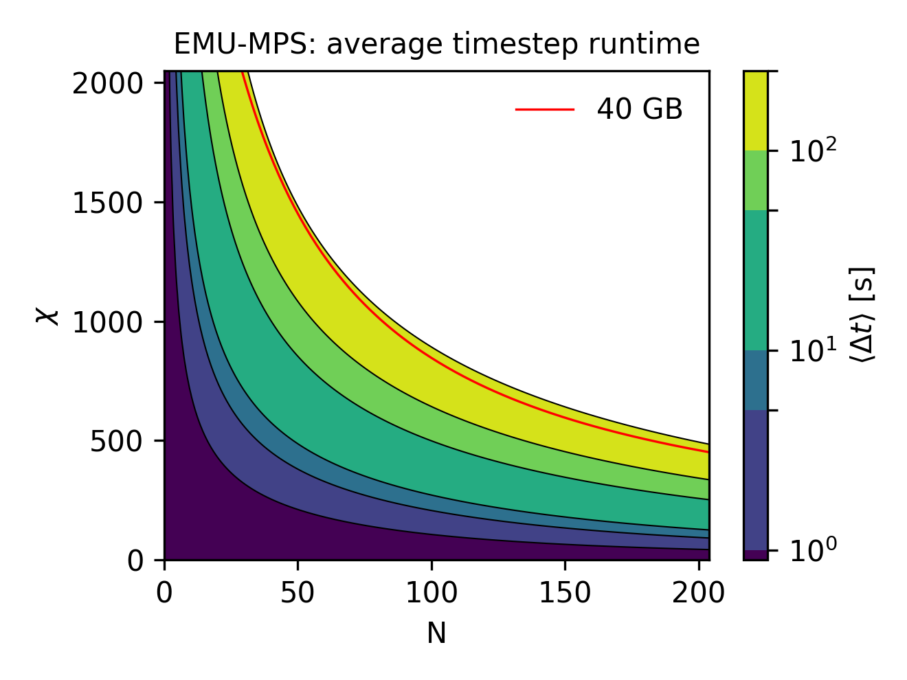
Superimposing the 40 GB hardware constrain derived in the previous section, it is easy to see that in worst-case scenario, a TDVP step will take roughly 250 seconds to be computed.